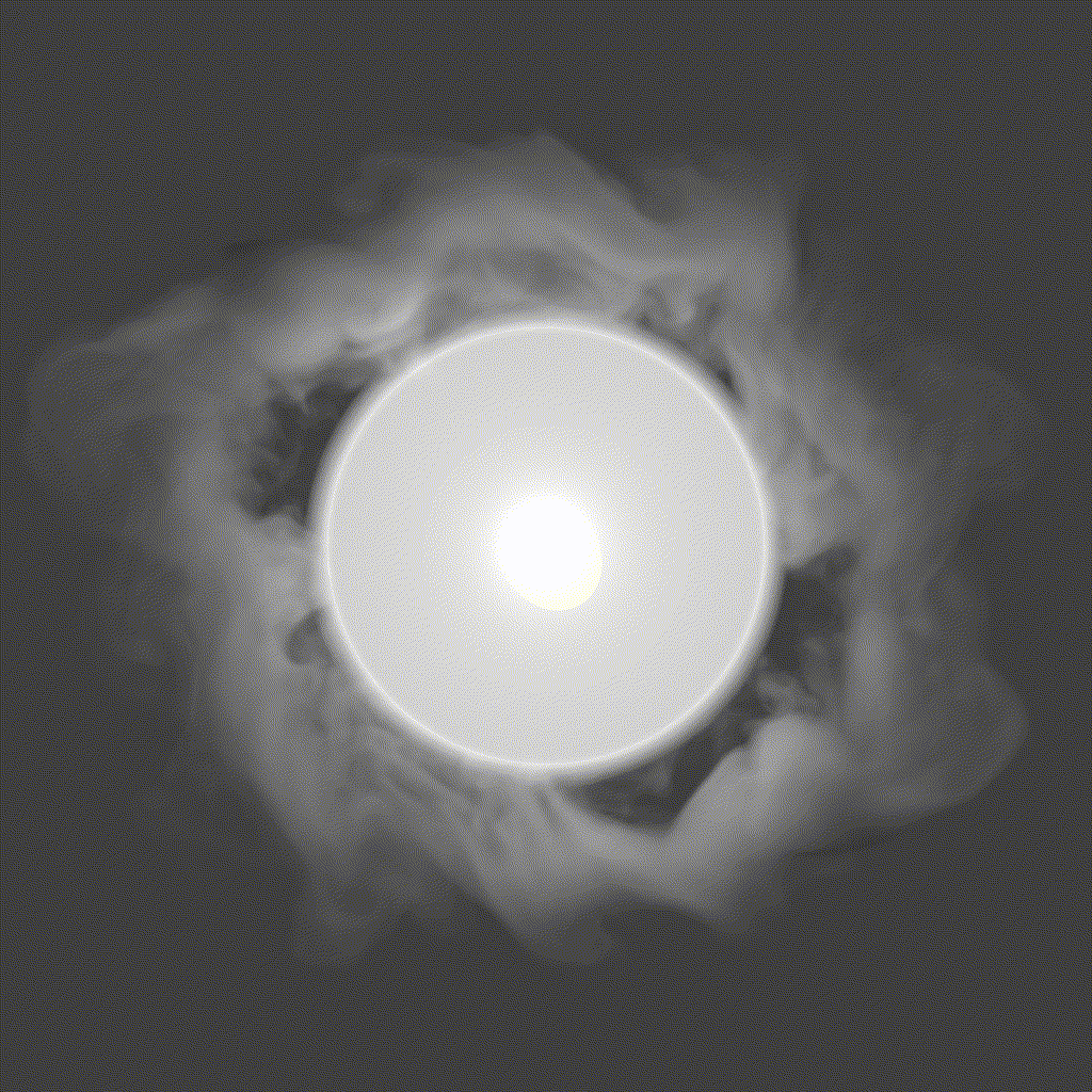
Creating seamless looping simulations for effects like smoke or fire is a common challenge in game development. While real-time volumetrics are becoming more prevalent, sprite sheets remain a practical solution. Traditional methods often result in visible seams or noticeable transitions, detracting from realism. This is particularly problematic when aiming for realistic effects, though such artifacts might be acceptable in stylized contexts.
I’ve developed a technique that, while not universally applicable, is particularly effective for generating smoke or fire simulations that appear consistent at both the start and end of the cycle. This approach enables the creation of a seamless volumetric effect presented as a sprite sheet comprising 64 frames.
![]()
On the homepage of my website, you can view an example of such a looped volumetric effect created using this sprite sheet method. Let’s delve into the process of crafting this effect.
Process Overview
The process began with a polygonal ring converted into a VDB. A sufficiently contrasting noise was applied to fill a designated area, accompanied by constant radial velocities. Additionally, two spheres were introduced, rotating to maximize velocity dispersion. A prolonged simulation was conducted to maintain consistent smoke movement, ensuring that, despite variations, the smoke remained within a specific spatial zone—a crucial condition for achieving a smooth loop.
Base Simulation Setup
The entire setup was executed using the standard SOP Pyro Solver in Houdini:
- Time Scale: Set to 0.25 to slow down the simulation.
- Resolution: Adjusted to ensure sufficient detail in a 512x512 image.
- Velocity Addition: Implemented in ‘pull’ mode for enhanced simulation stability.
- Disturbance: Applied delicately to introduce subtle variations.
- Advection: Utilized the BFECC (Back and Forth Error Compensation and Correction) method.
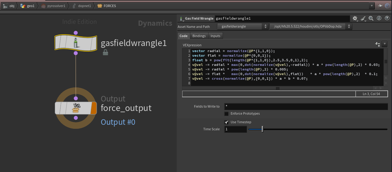
Within the solver, a Gas Field Wrangle was added for fine-tuning the smoke’s shape:
// Direction from center to each side of the ring
vector radial = normalize(@P * {1,1,0});

// Direction perpendicular to the ring's orientation
vector flat = normalize(@P * {0,0,1});

// Mask force by density
float a = sqrt(min(@density, 1));

// Mask for custom drag force
float b = pow(fit(length(@P * {1,1,0}), 2.5, 3.5, 0, 1), 2);

// Multiplier based on powered distance from center
float c = pow(length(@P), 2);

// Apply radial force (from outside to center)
// masked by density and current velocity directions
v@vel -= radial * max(0, dot(normalize(v@vel), -radial)) * a * c * 0.03;
v@vel -= radial * c * 0.005;

// Apply force to flatten the smoke ring
v@vel -= flat * max(0, dot(normalize(v@vel), flat)) * a * c * 0.1;

// Apply custom drag force (circular motion in backward direction)
v@vel -= cross(normalize(@P), {0,0,1}) * a * b * 0.07;
The simulation was run for an extended duration to allow the container to fill with velocities and stabilize, providing ample frames to select the most visually appealing segment. A 500-frame simulation was conducted.
Secondary Simulation (Creating the Loop)
The next step involved reviewing the simulation cache to identify a suitable 128-frame sequence with desirable motion characteristics. Two Time Shift nodes were then employed to swap the first and last halves of this sequence, aligning the transition precisely at the timeline’s midpoint.
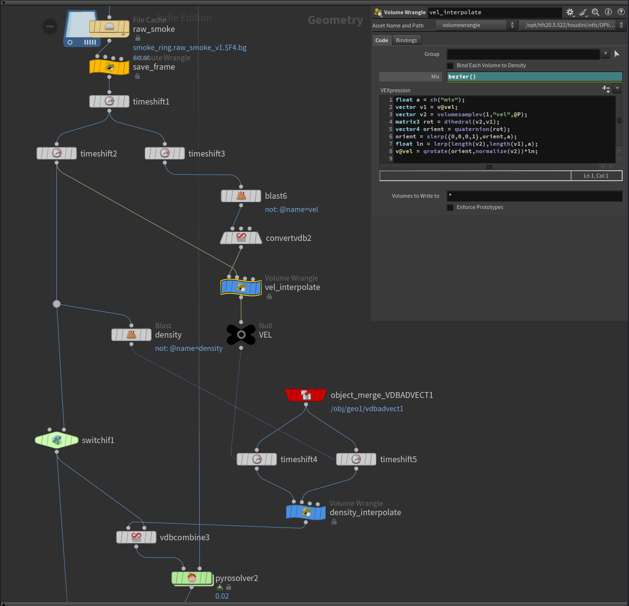
- timeshift1:
$F+350(aligns the start of the target range with the start frame) - timeshift2:
$F+63(moves the last part to the start) - timeshift3:
$F-64(moves the start part to the end) - blast6: Isolates the velocity grid.
- convertvdb2: Converts VDB to regular volumes.
- velocity_interpolate: Smoothly blends velocities between the two halves:
float a = ch("mix"); // Control parameter
// Retrieve current and second half velocities
vector v1 = v@vel;
vector v2 = volumesamplev(1, "vel", @P);

// Compute rotation matrix to align v1 with v2
matrix3 rot = dihedral(v2, v1);
// Convert matrix to quaternion and perform spherical interpolation
vector4 orient = quaternion(rot);
orient = slerp({0,0,0,1}, orient, a);

// Linearly interpolate vector lengths
float ln = lerp(length(v2), length(v1), a);
v@vel = qrotate(orient, normalize(v2)) * ln; // Export result
- timeshift4, timeshift5:
prim(-1,0,"frame",0)retrieves the original frame number. - density_interpolate:
float a = ch("mix");
float d1 = @density;
float d2 = volumesample(1, "density", @P);
// Simple linear interpolation of two input densities
@density = lerp(d2, d1, a);
- pyrosolver2: Similar to the first solver but without sourcing velocity or applying disturbance. The first part of the simulation serves as the starting source, with the same source used for all subsequent frames.
Within pyrosolver2, another gasfieldwrangle overrides velocity with values from the first simulation, added during the advection stage to prevent distortions.
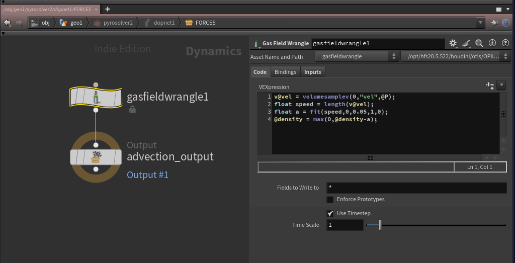
// read velocity from previous simulation
v@vel = volumesamplev(0,"vel",@P);

// make additional dissipation in zones, where velocity equals zero
// it helps to avoid strange looking stoped pieces of smoke
float speed = length(v@vel);
float a = fit(speed,0,0.05,1,0);
@density = max(0,@density-a);
- And last part fix some imperfections of the result shape and match seam frames:
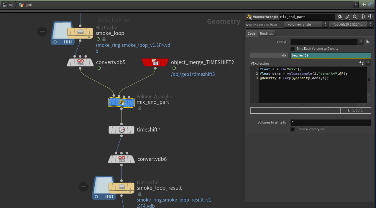
float a = ch("mix");
float dens = volumesample(1,"density",@P);
@density = lerp(@density,dens,a);
We have created a 64-frame looping smoke cache that appears completely seamless and maintains natural motion. This result can be watched endlessly.